Working with Workbooks
- Charles Bishop (Deactivated)
- Juliane Wetzel (Unlicensed)
- Judy Bergstresser (Deactivated)
In Datameer, you can create a workbook to get to new insights with your data. Inside the workbook, you can add additional data sources, change the column and sheet names, collapse columns, apply formulas, view workbook details, and more.
You can also copy workbooks, import worksheets from other workbooks, duplicate workbooks and worksheets, and exchange datasources.
Creating a Workbook
To create a workbook:
- Choose Workbooks from the + (plus) button or right-click in the navigation bar on the left side of the screen and select Create New > Workbook.
- From the File menu, select Add Data.
- Navigate to the folder where the data sources are located and select the name of the data source you want to use.
- Click Add Data.
When using data from a sheet in another workbook or an import job, the data from that source sheet is copied to the new sheet if the new sheet is marked as kept. In previous versions, the source sheet was referenced instead, which led to workbook data not being deleted by housekeeping.
The workbook is populated with a sample of data from that data source. To use data in Datameer, that data must be part of a data source. If you have a source of data you want to use for analysis, such as an Excel spreadsheet, you need to create a data source using that data, or have a system administrator create one for you.
Sample data and full data
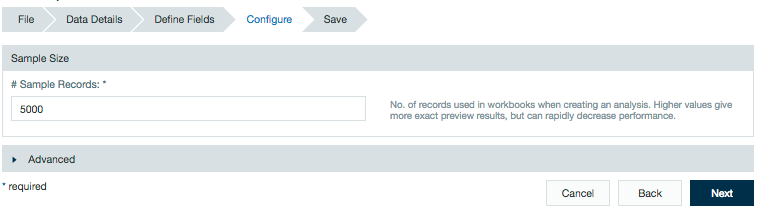
Data displayed in Datameer workbooks is a sampling of the full data from the source. When creating or editing an import job, file upload, or data link, you set the number of sample records to populate a workbook from the specific data source being used.
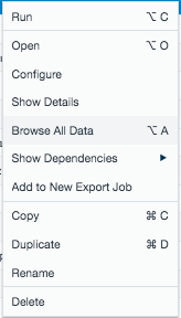
A data source added to a workbook displays the number of sample records configured for that source. When creating calculations in the workbook, those calculations are being applied only to the sample data until the workbook has run. After running a workbook, the calculations made in the workbook are applied to the full data and can be viewed or downloaded by right-clicking on the workbook and selecting Browse All Data.
The next time the workbook is opened after running, while the calculations have been applied to the full data, you still view the sample size configured from the data source.
Status notifications have been added to the bottom of workbook worksheets to show if the worksheet is displaying information based on sample or full data and if the worksheet is filtered.
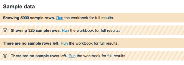
Sample data messages
If the worksheet's calculations are based only on sample data, the notification is orange. It tells you how many sample rows are being displayed in the worksheet and that you can run the workbook to display the sheet calculations based on the full data from the data source.
If the worksheet is displaying no information, this could be that none of the original sample data fits the criteria of the calculations. Running the workbook takes into account all current worksheet calculations and might bring in new sample data to populate the worksheet if data from the data source meet the calculation criteria.
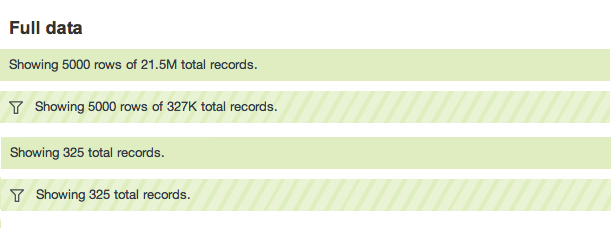
Full data messages
If the worksheet's calculations are based on the full data, the notification is green. It tells you how many sample rows are being displayed in the worksheet out of how many total records from the data source. If all the records of the source are being used, the status bar displays the total record count.
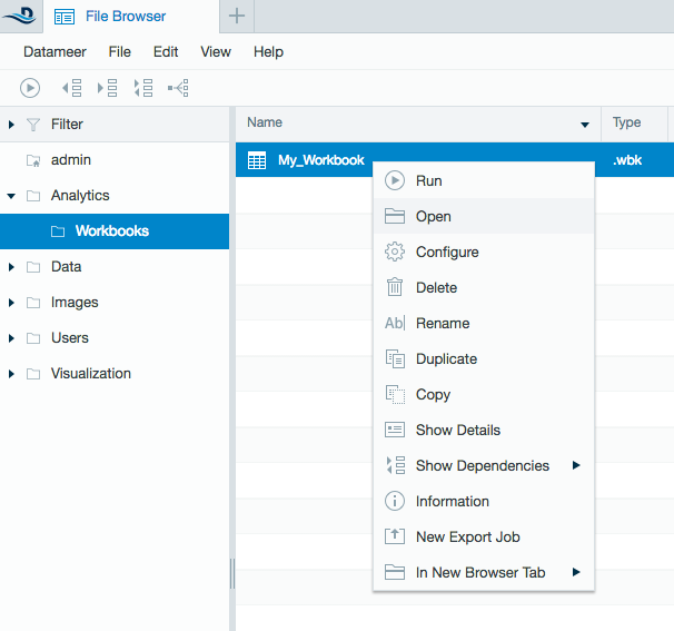
Opening Existing Workbooks
To open an existing workbook:
- On the File Browser tab, find the workbook you want to open.
- Highlight the workbook by clicking on it.
- Double-click to open or right-click on the highlighted workbook and select Open.
Opening a workbook using a URL
A workbook can be opened by a user with permissions to view the workbook by entering a URL into the browser.
There are two valid URLs that can open a workbook, using the ID or the path.
Workbook ID: http(s)://<server>:<port>/workbook/<wbkID>
Example: https://localhost:8080/workbook/25
Workbook path: http(s)://<server>:<port>/workbook?path=<path/to/workbook.wbk>
Example: https://localhost:8080/workbook?path=Users/Matthew/Seasonal_Earnings
Open a workbook to a specific worksheet: http(s)://<server>:<port>/workbook?path=<path/to/workbook.wbk>&sheet=<sheetName>
Example: https://localhost:8080/workbook?path=/Users/Matthew /Seasonal_Earnings.wbk&sheet=products
Opening a prior version of a workbook
Datameer gives you the option of saving previous versions of a workbook when it is run more than once. Learn more about optimizing your workbooks and data retention.
To open a prior version of a workbook:
- On the File Browser tab, find the workbook you want to open.
- Highlight the workbook by clicking on it.
- Right-click on the highlighted workbook and select Show Details.
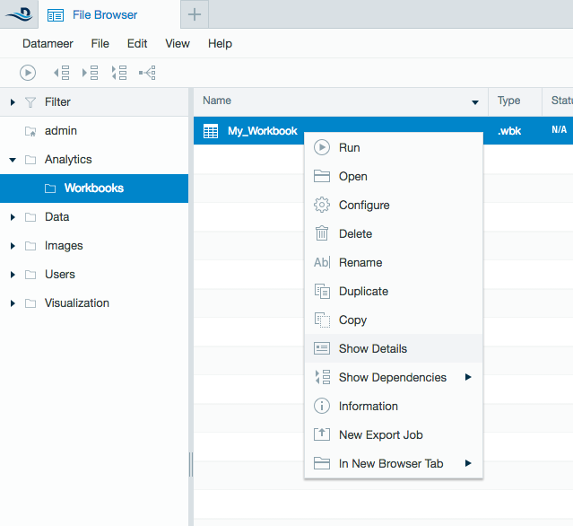
- Find the previously run workbook iteration in the Current Data section. Click the Show Data icon.
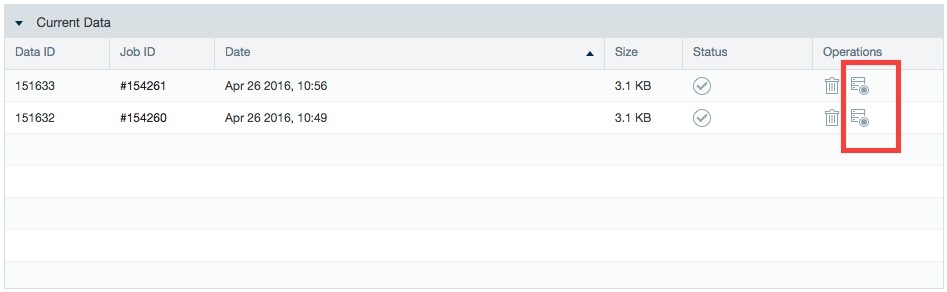
- From the Full Results page, you can open the workbook or download the data.
For convenience, other previous ran workbook iterations have a link.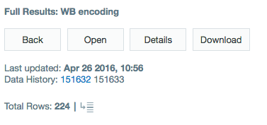
Adding Additional Data Sources
To add additional data sources to an existing workbook:
- From the File menu, choose Add Data or click the Add Data icon on the toolbar.
- Navigate to the folder where the data sources are located and select the name of the data source you want to use.
- Click Add Data.
- Repeat the previous steps for each data source you want to use.
For each data source you select, a tab is added to the workbook, containing a sample of data from that data source. You can add multiple data sources at the same time by holding the SHIFT button.
Exchanging Data Sources
You can exchange data sources to run a workbook on a different set of similar data, which is faster than recreating the workbook.
For example, you can run a workbook on data for each month by exchanging the data source to point to the data for the next month. Each datasource must have the same structure. Further analysis applies only to the new data after the exchange. This option is only available when the current data sheet uses a data source imported by adding data. The option isn't available for sheets created using filters, joins, sorts, external data sheets, or formulas. You must also have write permissions for this workbook to use this option.
To exchange data sources in an existing workbook:
- From the File menu, choose Exchange Data or click the Exchange Data icon on the toolbar.
- Navigate to the folder where the datasources are located and select the name of the data source you want to use.
- Click Exchange Data.
Errors might occur when exchanging data if column names have changed. On a joined sheet, original references to columns remain even if that column name doesn't exist in the new exchanged data. If this happens, replace the joined sheet reference with the updated column name from the exchanged data.
Working with Sheets and Columns
You can set up sheet names, resize columns, collapse and show columns, rename worksheets, import worksheets from other workbooks, and more.
Viewing sheets within a workbook
There are multiple ways to navigate between sheets within a workbook:
- Click the sheet tab you want to view a the bottom of the page.
- Select the Sheets menu and click the sheet you want to view.
- Click on the Sheet Dependencies button in the toolbar and switch between sheets by clicking on sheets that are dependent with each other.
Distinguishing different sheet types
There are eight different worksheet types in Datameer. Only the formula (Fx) worksheet type analyzes data using the formula bar or with the function wizard.
Renaming sheets
To change the name of a sheet:
- Right-click the sheet name and click Rename.
- Enter the new name and press Enter.
- To undo the change, right-click the name again and click Undo.
Deleting sheets in a workbook
To delete a sheet:
- Click the tab in the workbook that you want to delete.
- Right-click the tab and choose Delete.
- Click Delete.
Duplicating sheets in a workbook
You can duplicate workbook sheets. New sheets are named with the next available number appended to the sheet name.
To duplicate sheets in a workbook:
- Click the tab in the workbook.
- From the Workbook menu Sheets, select Duplicate Sheet or right-click the sheet tab and select Duplicate.
- In the Duplicate Worksheet, select the columns you want to copy to the new sheet and click Create Sheet Copy.
- If a sheet has actions applied to it, you have the option to copy both the logic and the data, or you can select the Copy data onlycheckbox to copy just the data.
As of Datameer v6.3
In addition to the raw data of a sheet with formulas, joins, sorts, or clustering, you can also copy the underlying logic and actions of a sheet into a new sheet.
Reordering sheets in a workbook
To reorder sheets within a workbook:
- Right-click the sheet tab.
- Select Move.
- Click the space between the current sheet tabs where you want the selected sheet to be placed.
Reordering columns in a workbook
To reorder columns in a sheet:
- Left-click and drag the column name to the desired position.
Displaying sheet dependency (graph overlay)
The graph overlay feature provides a graphic display of the currently selected sheet and any ingoing and outgoing sheets.
- View the sheet dependency overlay by clicking the Sheet Dependencies button in the toolbar. The currently selected sheet will be highlighted in the middle of the graph.
- To navigate between dependent sheets, click the sheet name located on the graphic overlay.
- To close the sheet dependencies overlay, click the toolbar button or click X on the current sheet.
Importing sheets
Importing sheets allows you to chain workbooks together.
To import sheets from one workbook into another workbook:
- Open the workbook you want to import the worksheet into.
- From the Workbook menu, select Add Data, or click the Add Data icon on the toolbar.
- First, select the workbook you want to use and click Add Data.
- Then select the sheets you want to import and click Add Data.
- The new worksheet tabs are added to the right of the existing worksheets.
Column names
When a user creates new columns using the Formula Builder, Datameer creates default column names based on the column name in the formula, and the formula type.
Column names in workbook sheets that are editable can be renamed. The status line just above the list of tabs indicates whether a particular sheet is editable.
Column names can only contain capital or lower-case characters, numbers, and underscores. A column name cannot begin with a number. Note that column names are case sensitive! For example, column names foo, FOO, FoO and fOO will be unique columns within the same worksheet.
As of Datameer 7.5
All column names, in all workbook sheet types, are case sensitive. This is a behavior change with version 7.5.
As of Datameer 7.2
Column names have a 255 character limit.
To edit a column name:
- Right-click on the column name and click Rename.
- Enter the new name and press Enter.
- To undo the change, right-click the name again and click Undo.
Resizing columns
To resize columns:
- Place the mouse between two column headings so the icon changes to a double-ended arrow.
- Drag the column marker to the desired width.
- Click to lock the width.
You can also double-click a column name to fully expand the column.
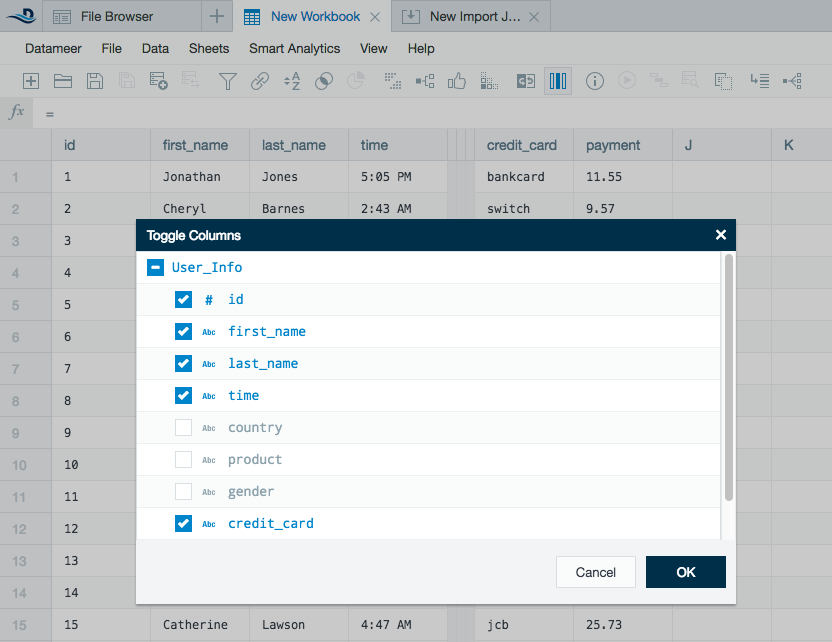
Hiding and expanding columns
To hide (collapse) a column, right-click the column name and select Hide Column.
Double-click the hidden column to bring it back into view.
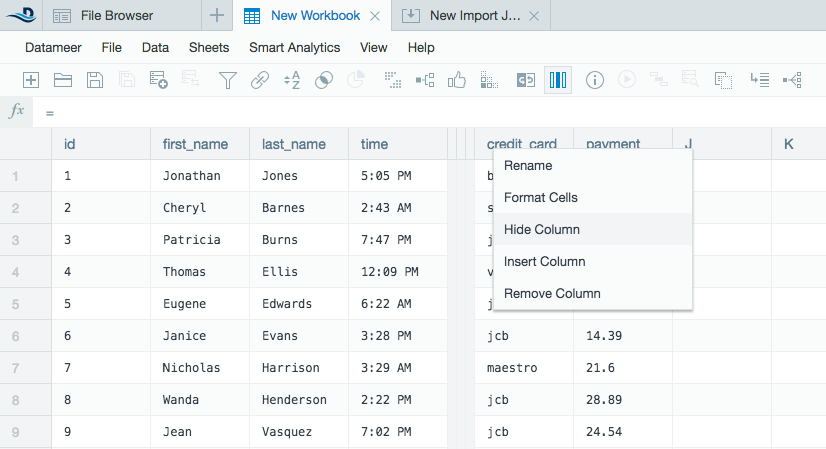
A toggle columns toolbar button displays all columns of the current worksheet. You can use this menu to show or hide columns as a batch process.
Inserting columns
To insert a new column:
- Right-click a column name.
Select Insert Column. A new column is added to the left of the chosen column.
Each workbook can contain a maximum of 702 columns.
Removing columns
To remove a column:
- Right-click a column name.
- Select Remove Column.
Cell context menu options
To access the cell context menu, right-click on a cell within a workbook.
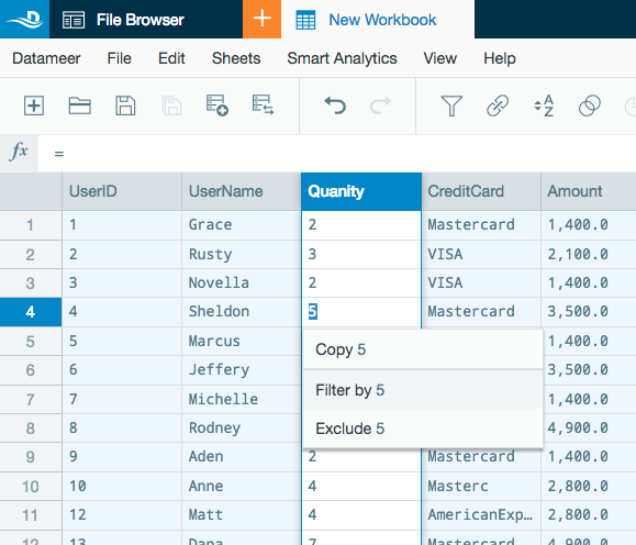
The cell context menu includes three options:
- Copy - Copy the cell value to the clipboard.
- Filter by - A shortcut to open the filter feature and auto completes the fields using the equals expression to filter for matches the cell's value.
- Exclude - A shortcut to open the filter feature and auto completes the fields using the does not equal expression to filter for matches that don't match the cell's value.
Splitting columns
Datameer 7.5 includes the option to split workbook string and list type column content by a selected delimiter. Several optional additional controls are available. Resulting column names are the original column name with a sequential number appended. For list columns, commas are the only delimiter and there will be one column per comma up to the column limit.
The split column operation can be updated as many times as you like until you have desired split configuration.
To split a column:
- Right-click on the column header of the column you want to split to open the context menu and select Split Column, or use the icon in the toolbar.
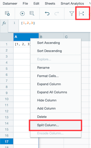
- In the Split to Columns dialog, the Input column will be selected automatically.
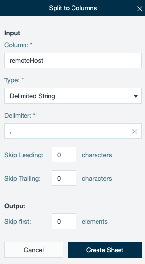
- For string columns, you must select the Type of column contents, either Delimited String or JSON Array String.
- For string columns, enter a Delimiter character.
The following optional controls are available:
- (Strings only) Use Skip Leading to enter the number of characters that will be ignored before the delimiter used to split the column.
- (Strings only) Use Skip Trailing to enter the number of characters that will be ignored after the specified number of columns are split.
- Use Skip first to ignore the first x number of elements, where elements are the characters between delimiters.
- Use Split into to specify a fixed number of columns into which data will be split.
- (JSON array only) When Catch additional data in overflow column is checked, if the number of original elements exceeds the number of specified output columns, the remaining elements will be kept and grouped into one column, in brackets.
- Use Drop additional elements to ignore all elements past the specified output columns.
- (Strings only) Use Trim Whitespace to delete any leading or trailing spaces and line breaks.
- (Strings only) Use Define Empty Value to specify what is substituted in if no existing data is split into the last columns (i.e. when the amount of data is smaller than the column limit.)
5. Optionally, enter a Column prefix that be prepended to the new column names.
6. Once you have entered your desired parameters, click Create Sheet.
7. A new SplitString or SplitList sheet opens containing the split columns.
If desired, you can use the Split tab in the Inspector to enter new split criteria. Click Update Sheet to apply changes.
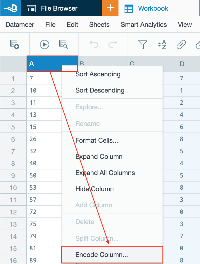
Encoding Columns
INFO
Column encoding performs ordinal, one-hot or binned encoding on column data which assigns a unique numeric value to each categorical or continuous value. Once applied, column encoding can be updated as needed until the desired results are achieved.
Columns with a high cardinality are not suited for ordinal/ binned encoding.
Column encoding provides a consistent view of prepared data which is especially helpful for teams working together on model building and testing activities.
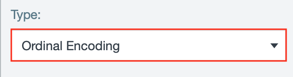
Ordinal Encoding
For ordinal encoding:
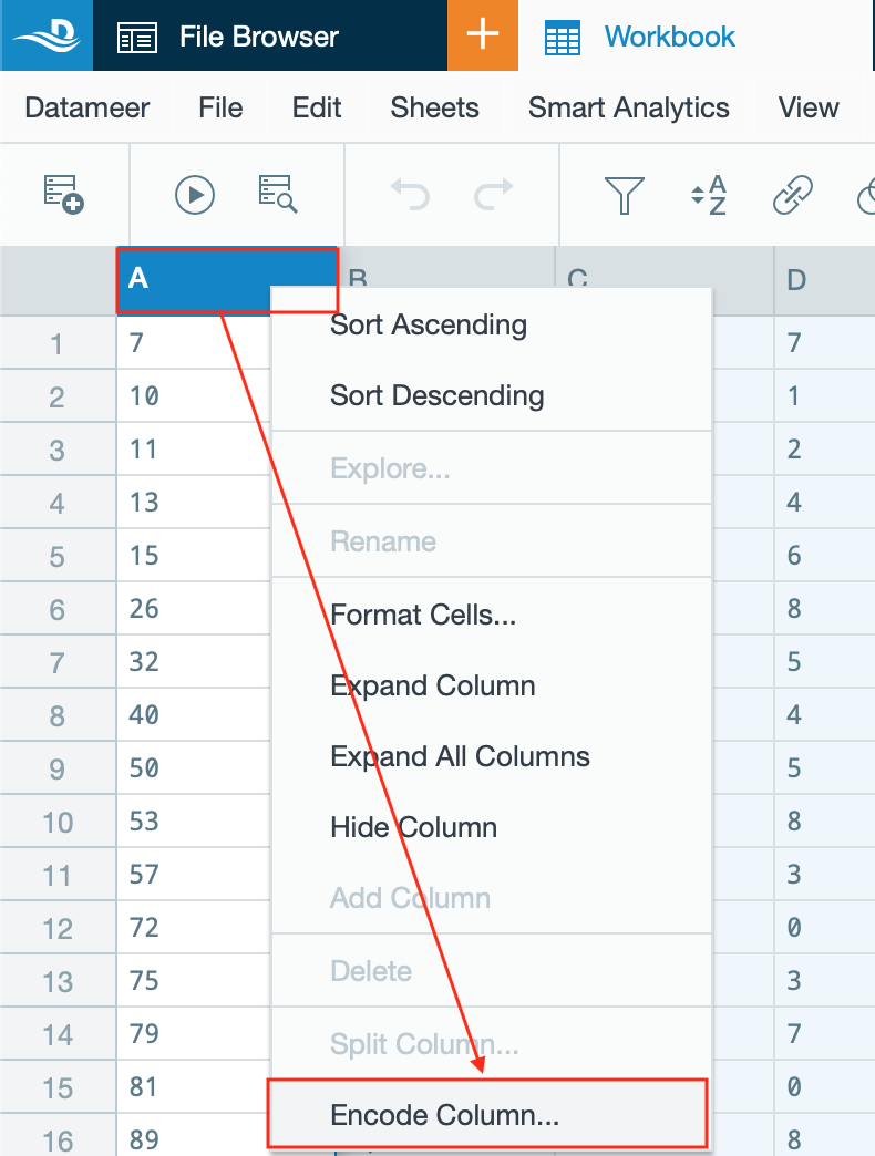
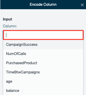
- Right-click on a column header and select "Encoding" or click on the "Encode Column" icon from the toolbar. The 'Encode Column' dialog is displayed on the right.
 or
or 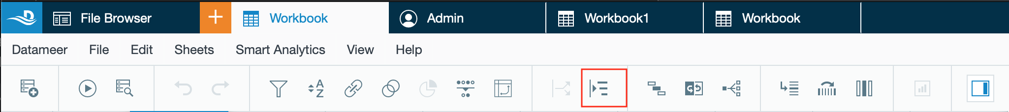
- If needed, change the column by entering the required column name in 'Column'.

- Select the encoding type "Ordinal Encoding" from the drop-down. Further selection options adapt to the needs.
- Decide how to deal with unknown values by clicking the required statement.
INFO: 'Drop Value' ignores values beyond the first 100 most frequent. 'Default Value' shows values, which can not be encoded.
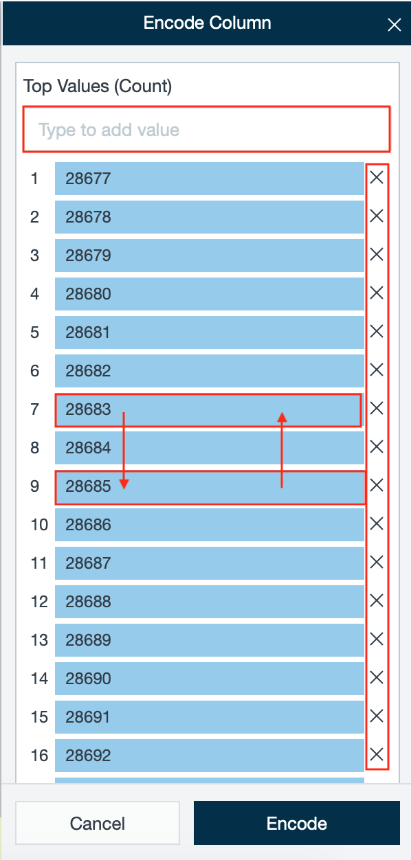
- View the top 32 values (by count).
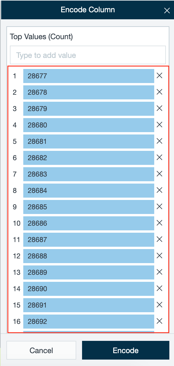
- If needed, add a new value in the blank field, change the order of the top values or delete single values.
- Confirm with "Encode". The encoding result is displayed in a new encoding sheet within the workbook. Ordinal Encoding is finished.
One-hot Encoding
For one-hot encoding:
- Right-click on a column header and select "Encoding" or click on the "Encode Column" icon from the toolbar. The 'Encode Column' dialog is displayed on the right.
 or
or 
- If needed, change the column by entering the required column name in 'Column'.
- Select the encoding type "1-Hot Encoding" from the drop-down. Further selection options adapt to the needs.
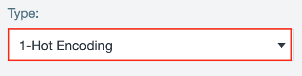
- Decide how to deal with unknown values by clicking the required statement.
INFO: 'Drop Value' ignores values beyond the first 100 most frequent. 'Include at last column' adds a new element to the list that encodes together all values beyond the 100 most frequent.
- Select the output format from the dropdown 'Output'.
INFO: 'As List' keeps all binary pairs together in a single column. 'As Column' creates binary pairs each in their own column.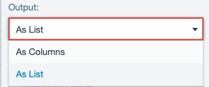
- View the top 32 values (by count).
- If needed, add a new value in the blank field, change the order of the top values or delete single values.
- Confirm with "Encode". The encoding result is displayed in a new encoding sheet within the workbook. One-hot encoding is finished.
Binned Encoding
For binned encoding:
- Right-click on a column header and select "Encoding" or click on the "Encode Column" icon from the toolbar. The 'Encode Column' dialog is displayed on the right. or
- If needed, change the column by entering the required column name in 'Column'.
- Select the encoding type "Binned Encoding" from the drop-down. Further selection options adapt to the needs.
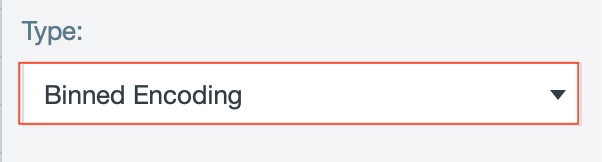
- Select the output format from the dropdown 'Output'.
INFO: 'As List' keeps all binary pairs together in a single column. 'Ordinal' encodes as ordinal numbers in a single column.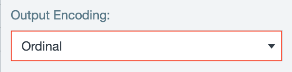
- View the default value distributions.
INFO: The graph changes according to the amount of dividers.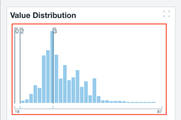
- Enter the required bin dividers to change the percentile size of the divider.
INFO: There are 3 dividers set as default, e.g. 'Divider 1' contains the 25% of the selected column values.
INFO: To delete a divider, click on "x" next to the required divider.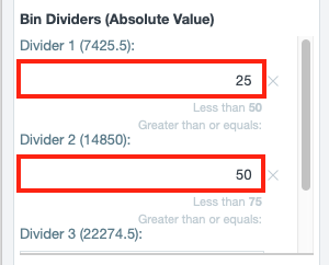
- If needed, click on "Add new Divider" to add a new divider.
INFO: Clinking the button adds an additional bucket, recalculates the percentile size and the corresponding absolute values.
- Confirm with "Encode". The encoding result is displayed in a new encoding sheet within the workbook. Binned encoding is finished.
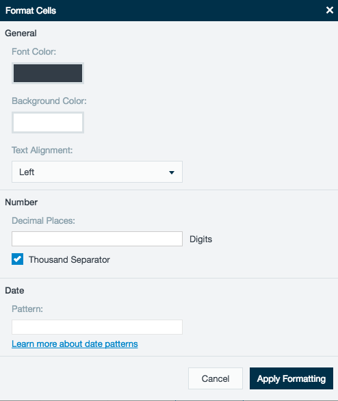
Formatting columns
To format the contents of a column:
- Right-click a column name.
- Select Format Cells.
- General
- Column text color
- Column background color
- Column text alignment (right, left, center)
- Numbers
- Thousands separator (comma to separate numbers by thousand)
- Select the amount of decimal places to display in the workbook
- Date
- Input a parse pattern to display the date. (The default doesn't display milliseconds)
Shading rows in a workbook
The worksheet highlights rows by each group series when a GROUPBY function is used. 
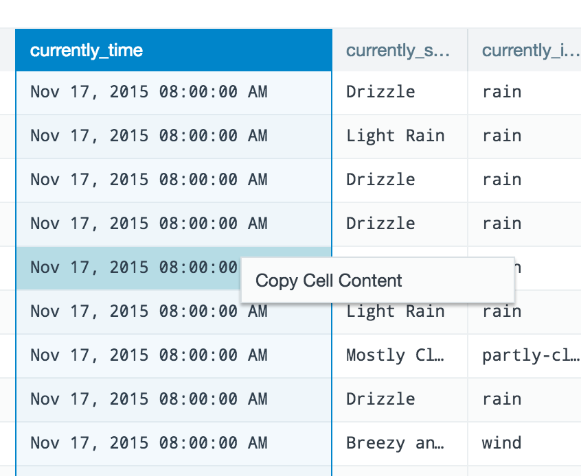
Copy cells
Double-click a cell to select it, and then right-click it and select Copy Cell Content to copy its contents to the browser's clipboard. This functionality doesn't work with the Safari browser.
Workbook inspector
The inspector gives you important information about the data of each column in your workbook. Use this feature for quick insights into the data that each of your columns contain.
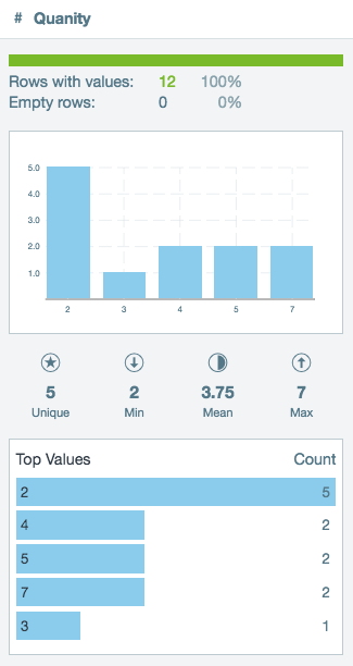
Information displayed in the column inspector:
- The name of the column being inspected.
- The number and percentage of valid and empty rows.
- A vertical bar chart displays all the different values and their frequency.
- Mousing over a bar in the chart displays the value(s) and count.
- If there are over 32 unique number type values, the bars group the values in bins.
- If there are over 32 unique non-number type values, the vertical bar chart is not displayed.
- The middle row of statistics displays the column's count of unique, minimum, mean, and maximum value.
- Mousing over a value displays the full value.
- Number and date field types are display all values. Other field types display only the unique count.
- The bottom horizontal bar chart displays the top unique values for the column and their respective counts.
- Mousing over a bar in the chart displays the value and count.
- Click the See more link below the bar chart to view additional column values in descending order.
As of Datameer 7.2
There are two tabs at the top of the workbook inspector. The inspector is separated at the worksheet level and column level.
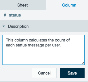
The worksheet level tab has a description box where text can be entered about each worksheet in the workbook.
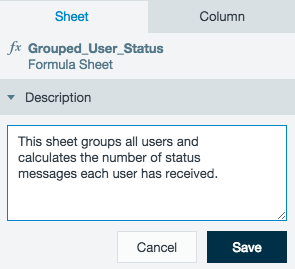
The column level tab has a description box where text can be entered about each column of a worksheet. Below the description box, the column information is as described above.
To open or close the workbook column inspector:
- Click View in the menu bar and select/unselect Inspector.
- Click the Inspector icon in the tool bar.
![]()
Deduplication
The deduplication feature eliminates duplicate/redundant data from your worksheet columns. This procedure can be performed across all columns of a worksheet or for specifically selected columns.
To deduplicate a column(s) in a worksheet:
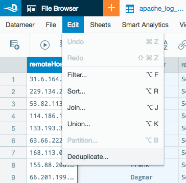
- From the Edit menu, click Deduplicate OR click the Deduplicate icon on the toolbar.
 or
or 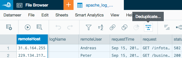
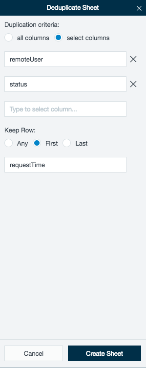
- The worksheet inspector changes to offer options on which columns you want to perform deduplication on.
Select the radio button for your choice between performing deduplication across all columns or select columns of the worksheet.- If you selected the all columns option, click the Create Sheet button at the bottom of the inspector to apply the deduplication process.
You workbook creates a new sheet titled TransformSheet. This sheet has purged any records that are a duplicate across all columns.
A new tab titled Deduplicate is located in your worksheet inspector.
Run the workbook to view the full results. - If you selected the select columns option, additional criteria fields appear.
Enter one or multiple columns to be used to deduplicate your data.
Optionally, you can select an additional column and choose to keep the first or last record of the deduplicated data.
Click the Create Sheet button at the bottom of the inspector to apply the deduplication process.
- If you selected the all columns option, click the Create Sheet button at the bottom of the inspector to apply the deduplication process.
A deduplicated sheet can be updated by clicking on the Deduplicate tab on the page inspector. Make a change to any option(s) and click Update Sheet.

Revert Actions
If you would like to revert an action that you performed in a workbook, you can use the Undo and Redo buttons available in the toolbar. By default, you can undo or redo the last two actions performed on a workbook that modify the workbook state in the database. These actions don't include changes such as font style or column size, as the workbook's state remains the same. You can also access these options through the Edit menu or using keyboard shortcuts (Cmd+Shift+Z for undo, Cmd+Shift+Z for redo). If the cursor is in a text field, using the keyboard shortcut reverts only the most recent changes in the text field, not the whole workbook.

Administrators can adjust the settings for these buttons in default.properties and system.properties. There, admins can edit the amount of time the history of a workbook is kept, the maximum number of actions a a user can revert, and how many workbooks can retain a history at the same time.
To make sure this functionality isn't causing performance issues, you can check various statistics about the memory usage and workbook states in <Datameer>/logs/workbook_undo.log. The log is set to record the following values separated by comma:
absoluteMemoryConsumption,absoluteMemoryUsageInBytes,generalMemoryUsage,historiesInUse,historyStatesInMemory,maxMemory,relativeUsageInPercent,usedMemory,usersWorking,workbooksInUse
All undo related actions are collected, but for memory performance, the system prints the values to the log once per minute.
Using Formulas
Formulas provide the ability to analyze your data in powerful ways.
Using the formula editor
The formula editor is located at the top of a worksheet within a workbook. Select a column on a worksheet and apply a formula with supported Datameer functions and operators.
Formulas can be added manually or using Datameer's Formula Builder. An auto-complete feature gives you the ability to visualize and complete formulas efficiently.
As of Datameer 7.2
The formula editor has multi-line functionality. Add more than one line when writing a formula so that it is easier to both read and write long and/or nested formulas.
Add additional lines by pressing Enter on your keyboard while in the editor. Submit your formulas by clicking the checkbox on the right of the editor or using the keyboard shortcut ⌘-Enter (mac) and Ctrl-Enter (win).
The multi-line editor can be expanded or collapsed by clicking and holding the edge of the formula bar and dragging your mouse.
Referencing worksheets and columns in the formula editor
A formula can only reference columns from it's own worksheet and one other worksheet in the workbook. Referencing columns from different worksheets is possible after a join sheet has first been created.
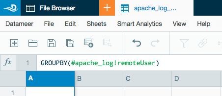
| Syntax for referencing a worksheet and column | ||
| Syntax | Example | |
|---|---|---|
| Worksheet | # | #apache_log |
| Column | ! | !remoteUser |
| Worksheet and column | #apache_log!remoteUser | |
Writing a function in the formula editor
Datameer's supported functions.
Enter a function name into the formula editor (case insensitive) with variables separated by a semicolon within parentheses.
Example: | Result explained |
|---|---|
| GE(#apache_log!status;400) | The Greater Than or Equal To function is being used comparing the "status" column from the "apache_log" worksheet |
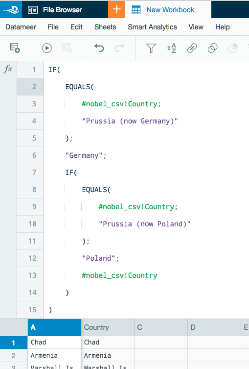
Writing nested functions in the formula editor
From the formula editor, you can enter functions and operators within functions.
| Example | Results explained |
|---|---|
| IF(EQUALS(#apache_log!status;400);"Bad Request";"other") | The IF function is being used with the Equals function as one of the variables. |
Creating formulas using the formula builder
You can create formulas on worksheets that are editable. When you click the data area of a column that has a formula associated with it, the formula displays above the workbook in the Fx bar. You can also create a new sheet and create formulas that reference fields from other sheets. Click the Fx button on the formula line to display the formula builder. (As of Datameer 7.2, the formula builder is located in the worksheet inspector.)
To create a formula using the Formula Builder:
- Click the Fx button on the formula line to access the formula builder.
- Select the categories in the left column to choose the type of function.
- Choose a function from the list on the right.
- Enter the argument or arguments shown for that function. You can click a sheet and select a column.
- Click the Plus icon to enter additional arguments (if supported).
- Click OK.
The resulting function displays next to the fx icon. To learn more, see using the Formula Builder.
To use operators in a formula:
- Click the data area in a column and the current formula if one exists displays above the workbook.
- Create or edit the formula using operators such as < or > or <= and press Enter.
To use regular expressions in a formula:
- Click the data area in a column and the current formula if one exists displays above the workbook.
- Create or edit the formula using regular expressions press Enter.
See Using Regular Expressions to see some examples. Datameer offers an API to extend the built-in formulas. See the Developer's Guide to learn more.
Editing formulas
To edit formulas:
- Click the data area in a column and the current formula displays above the workbook.
- Edit the formula and press Enter.
Using Variables Within Workbooks
Variable values can be used within the worksheet formula bar as well as other areas such as the filter worksheet feature.
Call a variable value using the following syntax:
${<variable name>}
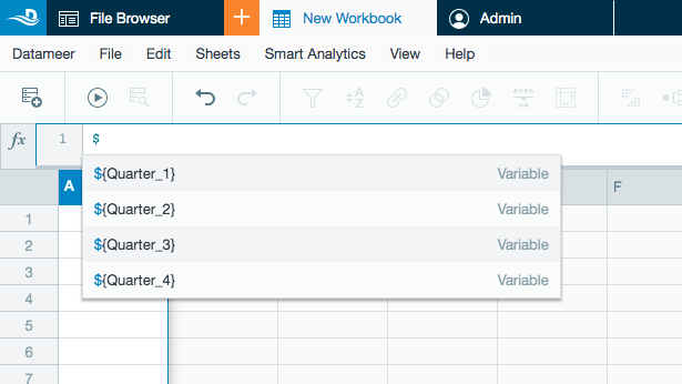
Variable values can be set by an administrator.
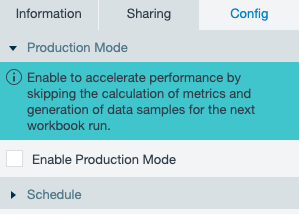
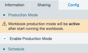
Workbook Production Mode
Production mode can be applied to a workbook to accelerate performance by skipping the calculation of metrics used for columnmetric, flip sheet displays and generation of data samples.
To launch production mode for a workbook:
- Within the file browser, select a workbook.
- Open the Config tab of the Inspector.
- Check Enable Production Mode.
Production mode is effective the next time the workbook is executed.
Completing Workbook Level Tasks
You can save workbooks, view or change workbook settings, link a workbook to multiple data sources, calculate a workbook, and more.
Saving workbooks
When you save a workbook, you also specify the workbook settings. If you don't know which settings to use, you can keep the default settings and you can change them later or the system administrator can set them. See Configuring Workbook Settings to learn more.
To save workbooks:
- From the File menu, select Save, or click the Save Workbook icon on the toolbar.
- Navigate to the folder where you want to save this workbook or choose to save the workbook in a new folder.
- Enter a name in the Save as field.
- Click Save.
If workbook settings need to be updated after saving, right-click on the workbook in the file browser and select Configure .
From the File menu, select Save As, or click the Save Workbook As icon on the toolbar.To save a copy of a workbook:
- Navigate to the folder where you want to save the workbook, enter a name, and click Save As.
Creating multiple workbooks
You can create multiple workbooks that reference the same data set:
- From the File menu, select New. Save your changes if needed.
- In the new workbook, from the File menu, select Add Data.
- Navigate to the data source you want to use and select the data source.
- Click Add Data.
Calculating a workbook
From the workbook you can calculate the workbook using the entire data set. Depending on the volume of data involved, this process might take awhile.
- From the Workbook menu, select Calculate or click the Calculate Full Workbook button on the toolbar. While the data is being calculated, you can click Abort if you want to calculate at a later time.
- Once the calculation is complete, the Full Data page opens.
- You can click Next button to view additional pages of data or click Go To Line and enter a line number to view a specific record.
- Click Edit to return to the workbook.
After making changes to an existing workbook, the next time the workbook is run, the changes are applied in the workbook calculation. Historical data before the change to the workbook isn't updated.
Viewing full results in a workbook
To view full results:
- From the Workbook menu, select View Full Results, or click the View Full Results icon on the toolbar.
- Click Open to view the data set in the worksheet view or click Next at the bottom of the table to view more records.
Going to line in a workbook
To go to a specific record while in the workbook:
- From the Workbook menu, select Go to Line or click the Go to Line button on the toolbar.
- Enter a line number to view a specific record and click Go.
Viewing workbook details
You can view information about the workbooks that you have open.
Workbook information gives general information about the current workbook, including:
- Name of the workbook
- Number of sheets the workbook contain
- The reprocessing schedule
- The last time the workbook was processed
- Notifications set for the workbook.
Sheet summary information gives advanced information on individual pages within the current workbook including the following:
| Sheet type | Sheet type | Description | Job path | Connection | Last executed | Kept | Partitioned | Formulas used | Filter source | Filter connector | Filter arguments | Join type | Join pairs | Sort source | Sort arguments | Sources of union |
|---|---|---|---|---|---|---|---|---|---|---|---|---|---|---|---|---|
| Source sheet | x | x | x | x | x | x | ||||||||||
| Formula sheet | x | x | x | x | ||||||||||||
| Filtered sheet | x | x | x | x | x | x | ||||||||||
| Joined sheet | x | x | x | x | x | |||||||||||
| Sorted sheet | x | x | x | x | ||||||||||||
| Union sheet | x | x | x | x |
To view workbook details:
- From the Workbook menu, select Workbook Info or click the Workbook Info button on the toolbar.
- The workbook information displays in a new window.
Changing workbook settings
You can set up the schedule of when a job runs when you create a workbook or you can change the schedule settings later. See Configuring Workbook Settings to learn more about scheduling.
Integrating workbook results with other systems
If you use other systems or BI tools, you can connect and consume results generated by Datameer workbooks so they can be leveraged for other processes or reporting mechanisms using the integration link.
The default limit for number of rows to download is 100,000, as this functionality is intended for small aggregated data sets. To adjust the record download limit, change the rest.download-data.records-max=100000 property in the <datameer_install>/conf/default.properties file. Setting the value to 0 unlocks the limit, but increasing the number could result in slower processing for the Datameer conductor. Your local system might also have download restrictions. If you want to download more than 100,000 rows, we suggest adjusting the number based on environmental variables from Datameer, your infrastructure, and external consuming tools.
Here is an example how it can be used in Power BI:
- Click Copy Integration Link in the Download dialog for full results page of a workbook. If you are using a browser that doesn't support copying to the clipboard, copy the provided URL instead.
.png?version=1&modificationDate=1517326678000&cacheVersion=1&api=v2&width=500&height=447)
- Go to Power BI Desktop and in the Get Data workflow, find Other > Web.
- Paste the URL in dialog and click OK.
- Select Basic authentication and enter your Datameer username and password for the environment linked previously and click Connect.
- On the next screen review and confirm the data to be loaded.
- Data is loaded and you can take full advantage of Power BI capabilities. You can also publish your Powe rBI dashboards and reports to Power BI Cloud maintaining reference to this Datameer connection.
Workbook Sharing Permissions and Security Settings
Only users with admin rights can set or change permissions.
To view sharing permissions and security settings for a workbook:
- Click the File Browser tab at the top of the page.
- Select the Workbooks folder.
- Click to highlight the workbook for which you want to edit permissions.
- Right-click the workbook and select Information or click the Information button on the tool bar.
- The sharing and full results sharing permissions can be found by clicking the Lock icon in the info box.
Sharing
Owner:
- The owner box shows the current owner of the workbook. The owner has view, edit, and run privileges. Changing the owner can only be completed by someone with administrative privileges.
Groups:
- User groups can be added to share the workbook. The administrator or owner of the workbook can set groups to view, edit, and run the workbook.
- By adding the view, edit, or run settings to All Users, the admin or user can set permissions for all users.
Full results sharing
- Full results sharing give the admin or owner the ability to give selected groups the ability to view the full data from the workbook.
- Only users that have access to the workbook in from the sharing section are eligible to view the full data of a workbook.
- In order to create infographics or export jobs from a workbook that you are not the owner of, you must have full results sharing permission.
Sharing workbooks with secure data sources
- Users that have permissions to view/edit a workbook but don't have permissions to view/edit the original data source being used in the workbook:
- Can't view the data source worksheet in the workbook.
- Can't view any worksheet in the workbook using data from the data source if the workbook hasn't yet run and/or the desired worksheets weren't kept.
- For workbook users to view/use worksheets that use data from a data source for which they don't have permissions, the workbook must first be run with the desired worksheets being kept.