Syntax
GROUP_HOLT_WINTERS(<number>;<number>;<number>;[<number>])
values: series values
α: data smoothing factor (between 0.0 and 1.0)
β: trend smoothing factor (between 0.0 and 1.0)
h: prediction range (how far the future should be predicted) - optional, default = 1
Description
This function computes Holt-Winters double exponential smoothing (non-seasonal) on a time series. Smoothing a time series helps remove random noise and leave the user with a general trend. Whereas in the simple moving average (GROUP_MOVING_AVERAGE) the past observations are weighted equally, exponential smoothing assigns exponentially decreasing weights over time. This gives a stronger weight to more recent values and can lead to better predictions.
This function can't be used referring to the same sheet, so make sure to use a different sheet than the value source sheet.
This is an aggregate function.
Example
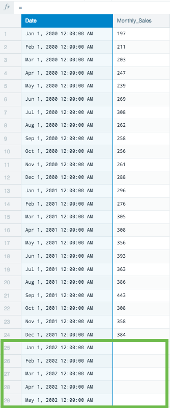
In the following example we have price values per month over a two year period. Let's try to predict the first 5 months of the third year using double exponential smoothing.
- Add five additional rows in the date column to better visualize the results for 5 months of future predictions.
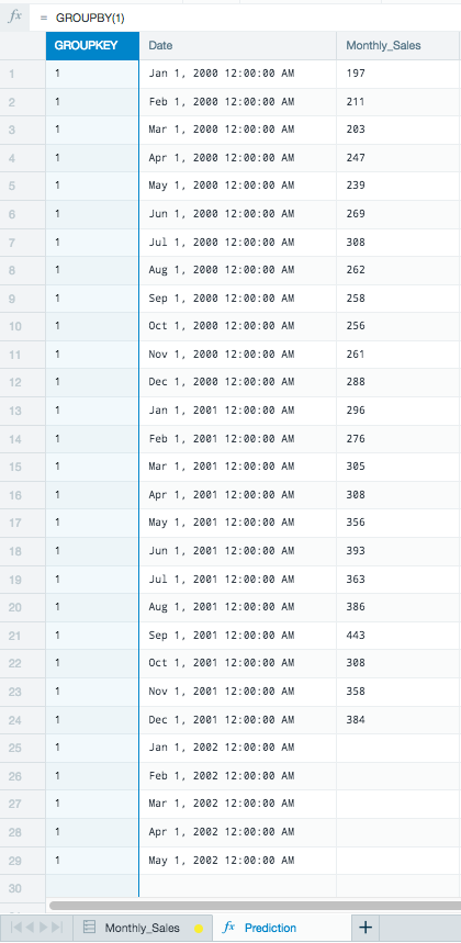
- Create a new worksheet in your workbook by duplicating the source sheet.
- Create a group key using GROUPBY(1).
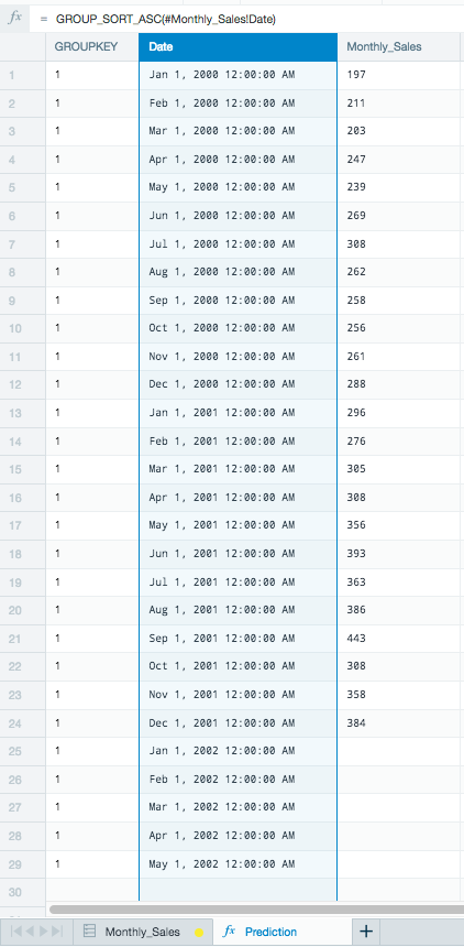
- Sort the timeline using GROUP_SORT_ASC(#Monthly_Sales!Date).
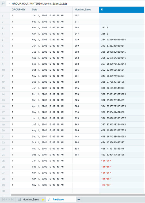
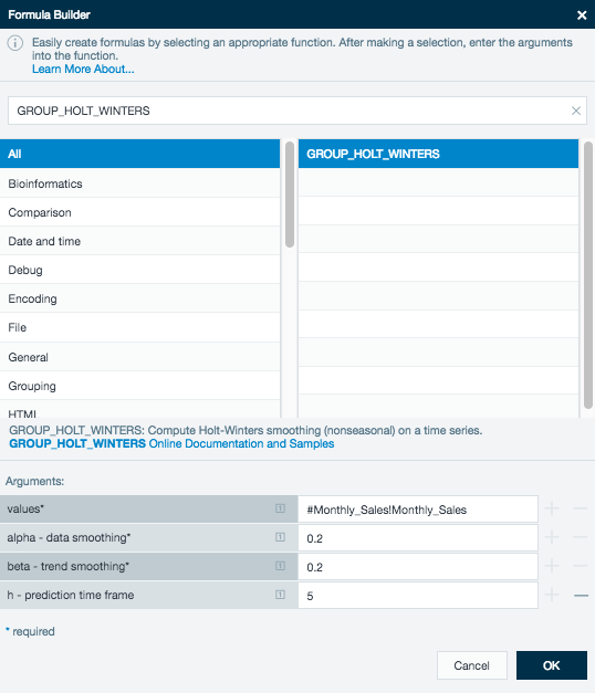
- Click an empty column to bring up the formula builder (As of Datameer v6.4, click the Fx button on the formula line to display the formula builder) and select GROUP_HOLT_WINTERS
. - Use the monthly sales column for the value's argument.
As this example uses a small data set, the alpha and beta arguments are set low at 0.2.
The Formula bar looks like this for your predicted values:
GROUP_HOLT_WINTERS(#Monthly_Sales;0.2;0.2;5)
There are two missing values for the rows, GROUP_HOLT_WINTERS needs these two values to compute the first prediction. Also, these predictions are 5 points in the future and currently don't match up with the date row.
To correct this, modify your Formula bar to:
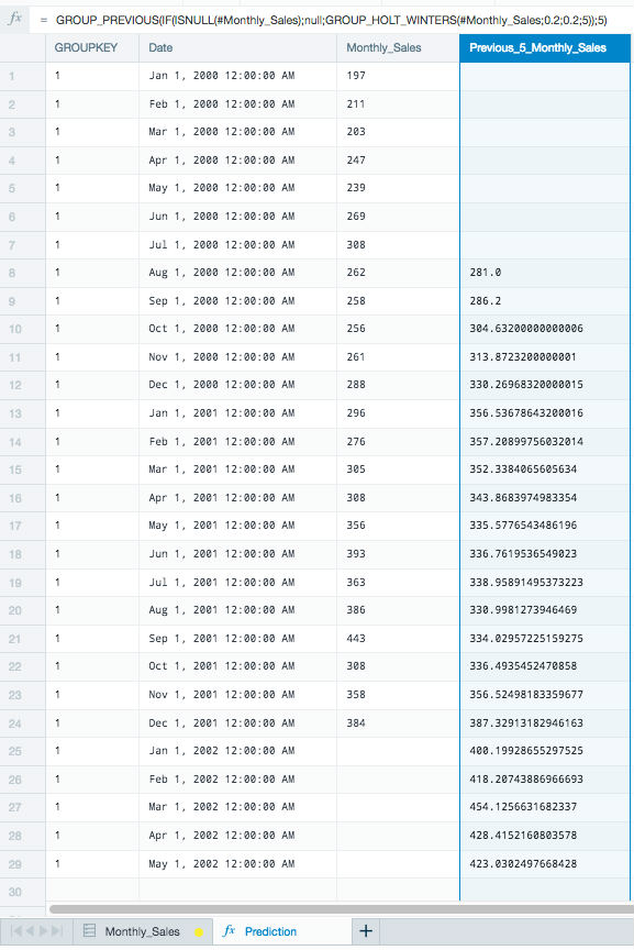
GROUP_PREVIOUS(IF(ISNULL(#Monthly_Sales);null;GROUP_HOLT_WINTERS(#Monthly_Sales;0.2;0.2;5));5)
This uses the functions GROUP_PREVIOUS to move the predictions 5 rows down to line up with the correct date. This also uses the function ISNULL to correct the error for the missing values in the rows with no values.
The sheet now displays the predicted data using the Holt-Winters exponential smoothing method.
Your finished workbook displays the full date range, the original values, and the predicted values.
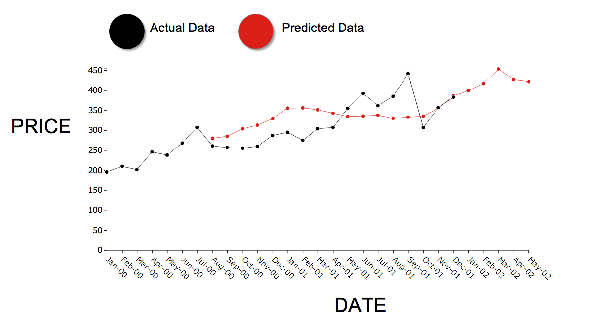
After having completed the workbook, use a Line Chart to visualize your new smoothed data predictions compared to your actual data.
